$$ \newcommand{\mybold}[1]{\boldsymbol{#1}} \newcommand{\trans}{\intercal} \newcommand{\norm}[1]{\left\Vert#1\right\Vert} \newcommand{\abs}[1]{\left|#1\right|} \newcommand{\bbr}{\mathbb{R}} \newcommand{\bbz}{\mathbb{Z}} \newcommand{\bbc}{\mathbb{C}} \newcommand{\gauss}[1]{\mathcal{N}\left(#1\right)} \newcommand{\chisq}[1]{\mathcal{\chi}^2_{#1}} \newcommand{\studentt}[1]{\mathrm{StudentT}_{#1}} \newcommand{\fdist}[2]{\mathrm{FDist}_{#1,#2}} \newcommand{\argmin}[1]{\underset{#1}{\mathrm{argmin}}\,} \newcommand{\projop}[1]{\underset{#1}{\mathrm{Proj}}\,} \newcommand{\proj}[1]{\underset{#1}{\mybold{P}}} \newcommand{\expect}[1]{\mathbb{E}\left[#1\right]} \newcommand{\prob}[1]{\mathbb{P}\left(#1\right)} \newcommand{\dens}[1]{\mathit{p}\left(#1\right)} \newcommand{\var}[1]{\mathrm{Var}\left(#1\right)} \newcommand{\cov}[1]{\mathrm{Cov}\left(#1\right)} \newcommand{\sumn}{\sum_{n=1}^N} \newcommand{\meann}{\frac{1}{N} \sumn} \newcommand{\cltn}{\frac{1}{\sqrt{N}} \sumn} \newcommand{\trace}[1]{\mathrm{trace}\left(#1\right)} \newcommand{\diag}[1]{\mathrm{Diag}\left(#1\right)} \newcommand{\grad}[2]{\nabla_{#1} \left. #2 \right.} \newcommand{\gradat}[3]{\nabla_{#1} \left. #2 \right|_{#3}} \newcommand{\fracat}[3]{\left. \frac{#1}{#2} \right|_{#3}} \newcommand{\W}{\mybold{W}} \newcommand{\w}{w} \newcommand{\wbar}{\bar{w}} \newcommand{\wv}{\mybold{w}} \newcommand{\X}{\mybold{X}} \newcommand{\x}{x} \newcommand{\xbar}{\bar{x}} \newcommand{\xv}{\mybold{x}} \newcommand{\Xcov}{\Sigmam_{\X}} \newcommand{\Xcovhat}{\hat{\Sigmam}_{\X}} \newcommand{\Covsand}{\Sigmam_{\mathrm{sand}}} \newcommand{\Covsandhat}{\hat{\Sigmam}_{\mathrm{sand}}} \newcommand{\Z}{\mybold{Z}} \newcommand{\z}{z} \newcommand{\zv}{\mybold{z}} \newcommand{\zbar}{\bar{z}} \newcommand{\Y}{\mybold{Y}} \newcommand{\Yhat}{\hat{\Y}} \newcommand{\y}{y} \newcommand{\yv}{\mybold{y}} \newcommand{\yhat}{\hat{\y}} \newcommand{\ybar}{\bar{y}} \newcommand{\res}{\varepsilon} \newcommand{\resv}{\mybold{\res}} \newcommand{\resvhat}{\hat{\mybold{\res}}} \newcommand{\reshat}{\hat{\res}} \newcommand{\betav}{\mybold{\beta}} \newcommand{\betavhat}{\hat{\betav}} \newcommand{\betahat}{\hat{\beta}} \newcommand{\betastar}{{\beta^{*}}} \newcommand{\bv}{\mybold{\b}} \newcommand{\bvhat}{\hat{\bv}} \newcommand{\alphav}{\mybold{\alpha}} \newcommand{\alphavhat}{\hat{\av}} \newcommand{\alphahat}{\hat{\alpha}} \newcommand{\omegav}{\mybold{\omega}} \newcommand{\gv}{\mybold{\gamma}} \newcommand{\gvhat}{\hat{\gv}} \newcommand{\ghat}{\hat{\gamma}} \newcommand{\hv}{\mybold{\h}} \newcommand{\hvhat}{\hat{\hv}} \newcommand{\hhat}{\hat{\h}} \newcommand{\gammav}{\mybold{\gamma}} \newcommand{\gammavhat}{\hat{\gammav}} \newcommand{\gammahat}{\hat{\gamma}} \newcommand{\new}{\mathrm{new}} \newcommand{\zerov}{\mybold{0}} \newcommand{\onev}{\mybold{1}} \newcommand{\id}{\mybold{I}} \newcommand{\sigmahat}{\hat{\sigma}} \newcommand{\etav}{\mybold{\eta}} \newcommand{\muv}{\mybold{\mu}} \newcommand{\Sigmam}{\mybold{\Sigma}} \newcommand{\rdom}[1]{\mathbb{R}^{#1}} \newcommand{\RV}[1]{\tilde{#1}} \def\A{\mybold{A}} \def\A{\mybold{A}} \def\av{\mybold{a}} \def\a{a} \def\B{\mybold{B}} \def\S{\mybold{S}} \def\sv{\mybold{s}} \def\s{s} \def\R{\mybold{R}} \def\rv{\mybold{r}} \def\r{r} \def\V{\mybold{V}} \def\vv{\mybold{v}} \def\v{v} \def\U{\mybold{U}} \def\uv{\mybold{u}} \def\u{u} \def\W{\mybold{W}} \def\wv{\mybold{w}} \def\w{w} \def\tv{\mybold{t}} \def\t{t} \def\Sc{\mathcal{S}} \def\ev{\mybold{e}} \def\Lammat{\mybold{\Lambda}} $$

Interpreting the coefficients and R output

$\,$

library(tidyverse)
library(sandwich)

theme_update(text = element_text(size=24))
options(repr.plot.width=12, repr.plot.height=6)

── Attaching core tidyverse packages ──────────────────────────────────────────────────────────────────────────────────────────────────────────────────────────────────────────────────────────────────────────────────────────────────────────────────────────── tidyverse 2.0.0 ──
✔ dplyr     1.1.2     ✔ readr     2.1.4
✔ forcats   1.0.0     ✔ stringr   1.5.0
✔ ggplot2   3.4.2     ✔ tibble    3.2.1
✔ lubridate 1.9.2     ✔ tidyr     1.3.0
✔ purrr     1.0.1     
── Conflicts ────────────────────────────────────────────────────────────────────────────────────────────────────────────────────────────────────────────────────────────────────────────────────────────────────────────────────────────────────────────── tidyverse_conflicts() ──
✖ dplyr::filter() masks stats::filter()
✖ dplyr::lag()    masks stats::lag()
ℹ Use the conflicted package (<http://conflicted.r-lib.org/>) to force all conflicts to become errors

install <- FALSE

# https://avehtari.github.io/ROS-Examples/examples.html
if (install) {
    install.packages("rprojroot")
    remotes::install_github("avehtari/ROS-Examples", subdir="rpackage")    
}

library(rosdata)
data(kidiq)

head(kidiq)

A data.frame: 6 × 5
	kid_score	mom_hs	mom_iq	mom_work	mom_age
	<int>	<int>	<dbl>	<int>	<int>
1	65	1	121.11753	4	27
2	98	1	89.36188	4	25
3	85	1	115.44316	4	27
4	83	1	99.44964	3	25
5	115	1	92.74571	4	27
6	98	0	107.90184	1	18

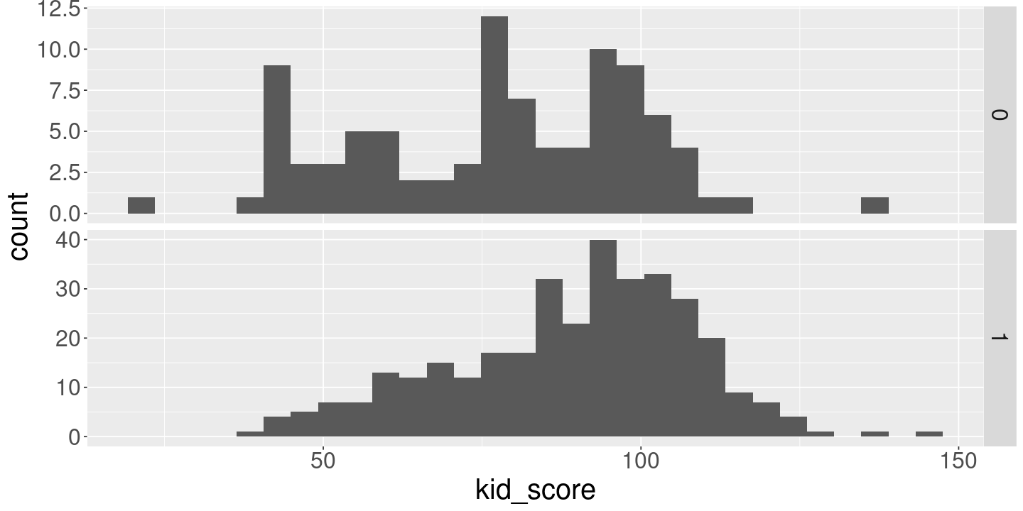
fit_hs <- lm(kid_score ~ 1 + mom_hs, kidiq)
print(fit_hs)

ggplot(kidiq) +
    geom_histogram(aes(x=kid_score)) +
    facet_grid(mom_hs ~ ., scales="free")


Call:
lm(formula = kid_score ~ 1 + mom_hs, data = kidiq)

Coefficients:
(Intercept)       mom_hs  
      77.55        11.77

`stat_bin()` using `bins = 30`. Pick better value with `binwidth`.

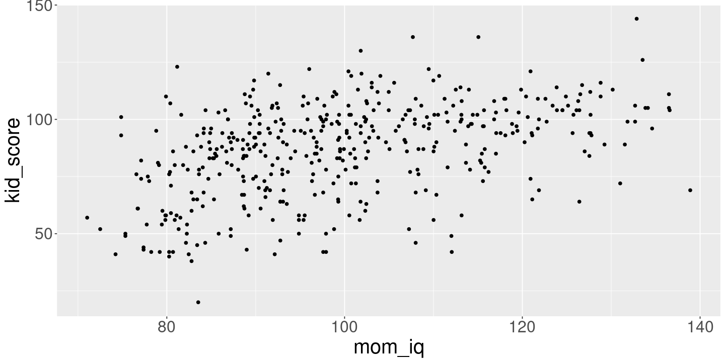
Kid score = $\beta_0$ + $\beta_1$ mom_iq

fit_iq <- lm(kid_score ~ mom_iq, kidiq)
print(fit_iq)

ggplot(kidiq) +
    geom_point(aes(x=mom_iq, y=kid_score))


Call:
lm(formula = kid_score ~ mom_iq, data = kidiq)

Coefficients:
(Intercept)       mom_iq  
      25.80         0.61

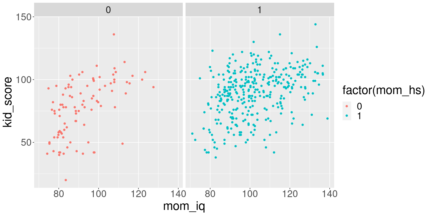
fit_hs_iq <- lm(kid_score ~ mom_hs + mom_iq, kidiq)
ggplot(kidiq) +
    geom_point(aes(x=mom_iq, y=kid_score, color=factor(mom_hs), group=mom_hs)) +
    facet_grid(. ~ mom_hs)

print(fit_hs_iq)


Call:
lm(formula = kid_score ~ mom_hs + mom_iq, data = kidiq)

Coefficients:
(Intercept)       mom_hs       mom_iq  
    25.7315       5.9501       0.5639

print(fit_hs)
print(fit_iq)
print(fit_hs_iq)


Call:
lm(formula = kid_score ~ 1 + mom_hs, data = kidiq)

Coefficients:
(Intercept)       mom_hs  
      77.55        11.77  


Call:
lm(formula = kid_score ~ mom_iq, data = kidiq)

Coefficients:
(Intercept)       mom_iq  
      25.80         0.61  


Call:
lm(formula = kid_score ~ mom_hs + mom_iq, data = kidiq)

Coefficients:
(Intercept)       mom_hs       mom_iq  
    25.7315       5.9501       0.5639

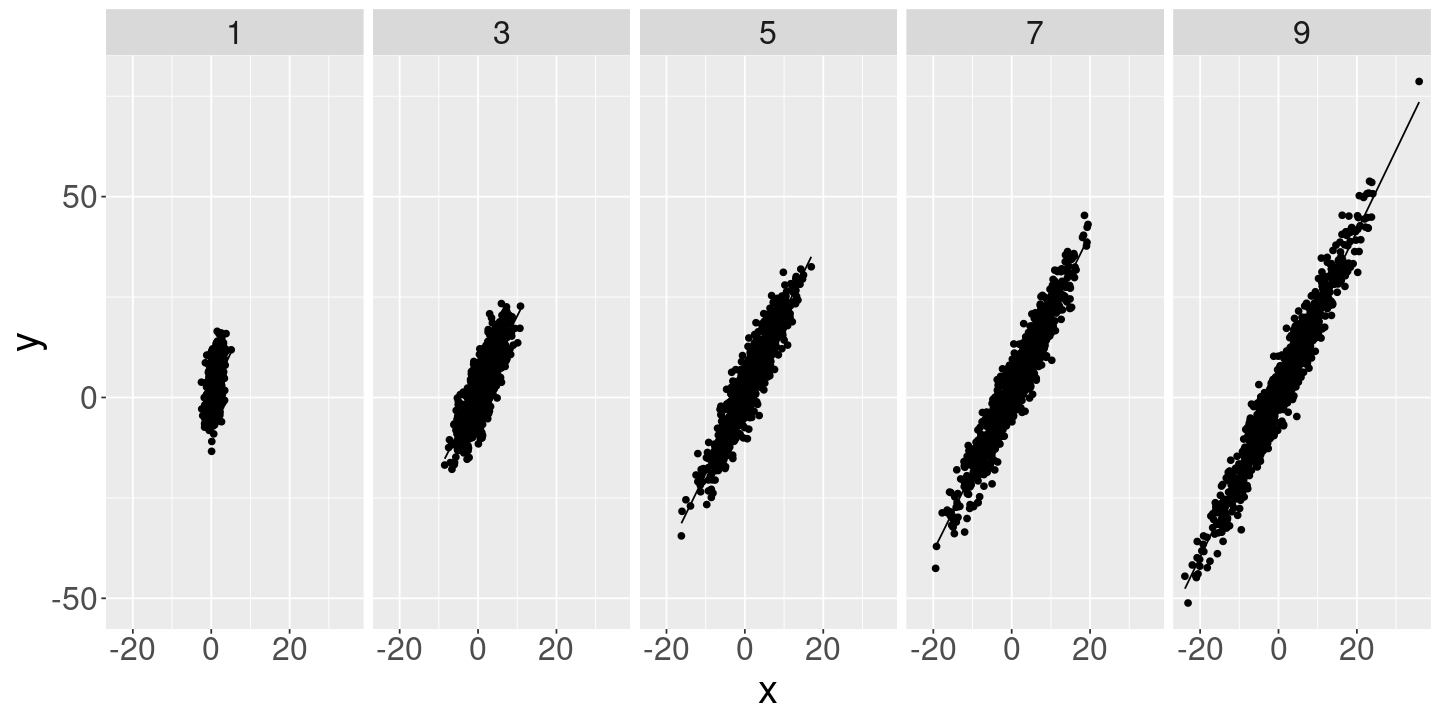
Simulations

Let’s look at the behavior of the standard errors of $\betahat_1$ when regressing $\y_n \sim \beta_0 + \beta_1 \x_n$, where $\var{\res_n} = \sigma^2$ and $\var{\x_n} = \sigma_x^2$.

sigma_x_vals <- seq(1.0, 10, by=2)
sigma_eps <- 4.0

n_obs <- 1000

beta_0 <- 1.0
beta_1 <- 2.0

fits <- list()
df_comb <- data.frame()
fits <- data.frame()
for (sigma_x in sigma_x_vals) {
    x <- rnorm(n_obs, mean=1.0, sd=sigma_x)
    eps <- rnorm(n_obs, mean=0, sd=sigma_eps)
    y <- beta_0 + beta_1 * x + eps
    df <- data.frame(y=y, x=x, eps=eps, sigma_x=sigma_x)
    fit <- lm(y ~ 1 + x, df)
    coeffs <- summary(fit)$coefficients["x", , drop=FALSE] %>% as.data.frame() %>% mutate(sigma_x=sigma_x)
    fits <- bind_rows(fits, coeffs)
    df <- df %>% mutate(y_pred=fit$fitted.values)
    df_comb <- bind_rows(df_comb, df)
}

ggplot(df_comb) +
    geom_point(aes(x=x, y=y)) +
    geom_line(aes(x=x, y=y_pred)) +
    facet_grid(~ sigma_x)

fits

A data.frame: 2 × 5
	Estimate	Std. Error	t value	Pr(>\|t\|)	sigma_x
	<dbl>	<dbl>	<dbl>	<dbl>	<dbl>
x...1	1.983005	0.131168439	15.118	1.193266e-46	1
x...2	1.998115	0.004886705	408.888	0.000000e+00	26