Regression to the mean
Goals
- Gain intuition for the phenomenon of regression to the mean
- Everyday intuition
- The asymmetry of OLS
- The effect on regression of noise in the regressors
Regression to the mean
Read Statistics (Freedman, Pisani and Purves) chapter 10 section 4.
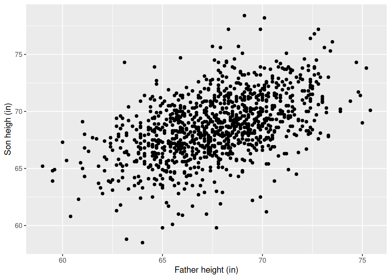
Fathers and sons
We expect that a son is roughly the same height as his father. But if we run the regression
reg <- lm(Son ~ 1 + Father, pearson_df)
print(summary(reg))
Call:
lm(formula = Son ~ 1 + Father, data = pearson_df)

Residuals:
    Min      1Q  Median      3Q     Max
-8.8910 -1.5361 -0.0092  1.6359  8.9894

Coefficients:
            Estimate Std. Error t value Pr(>|t|)
(Intercept) 33.89280    1.83289   18.49   <2e-16 ***
Father       0.51401    0.02706   19.00   <2e-16 ***
---
Signif. codes:  0 '***' 0.001 '**' 0.01 '*' 0.05 '.' 0.1 ' ' 1

Residual standard error: 2.438 on 1076 degrees of freedom
Multiple R-squared:  0.2512,    Adjusted R-squared:  0.2505
F-statistic: 360.9 on 1 and 1076 DF,  p-value: < 2.2e-16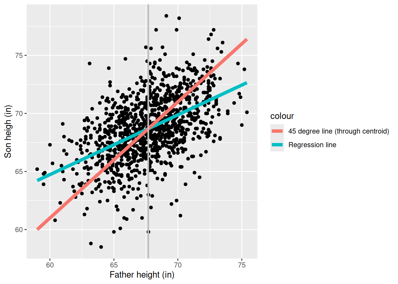
Are sons shrinking over time? In fact, note that we can run the regression the other way and get a similar result:
reg_reversed <- lm(Father ~ 1 + Son, pearson_df)
print(summary(reg_reversed))
Call:
lm(formula = Father ~ 1 + Son, data = pearson_df)

Residuals:
    Min      1Q  Median      3Q     Max
-7.3309 -1.6468  0.0634  1.6200  7.1589

Coefficients:
            Estimate Std. Error t value Pr(>|t|)
(Intercept) 34.12494    1.76815    19.3   <2e-16 ***
Son          0.48864    0.02572    19.0   <2e-16 ***
---
Signif. codes:  0 '***' 0.001 '**' 0.01 '*' 0.05 '.' 0.1 ' ' 1

Residual standard error: 2.377 on 1076 degrees of freedom
Multiple R-squared:  0.2512,    Adjusted R-squared:  0.2505
F-statistic: 360.9 on 1 and 1076 DF,  p-value: < 2.2e-16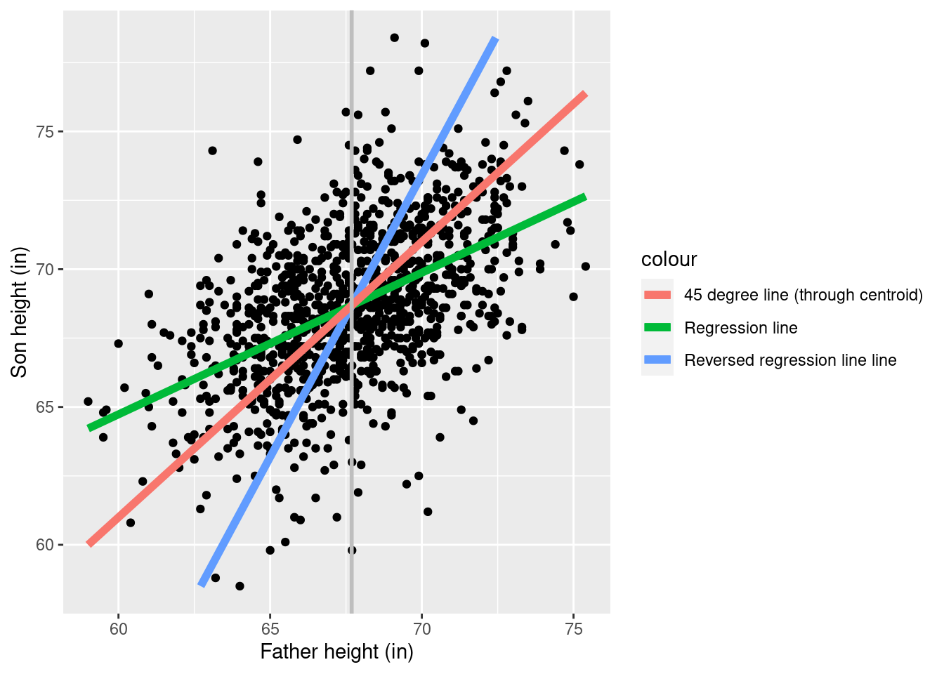
Of course it cannot be the case that fathers are smaller than sons and sons are smaller than fathers.
What is going on? This is an example of two common phenoena:
- Regression to the mean
- Errors in regressors
The asymmetry of regression
Consider this thought experiment. Imagine a dataset where fathers’ and sons’ heights are totally unrelated. It might look like the left plot below. It seems clear that, if we regressed \(\textrm{Son height} ~ 1 + \textrm{Father height}\) on this totally unrelated data, we should get a slope of \(0\). Conversely, if son height is exactly equal to father height, then the data should look like the right plot, and we should get a slope of \(1\).
grid.arrange(
ggplot(data.frame(Father=rnorm(500), Son=rnorm(500))) +
  geom_point(aes(x=Father, y=Son)) +
  xlab("Father height (in)") + ylab("Son height (in)")
,
ggplot(data.frame(Father=rnorm(500))) +
  geom_point(aes(x=Father, y=Father)) +
  xlab("Father height (in)") + ylab("Son height (in)"),
  ncol=2
)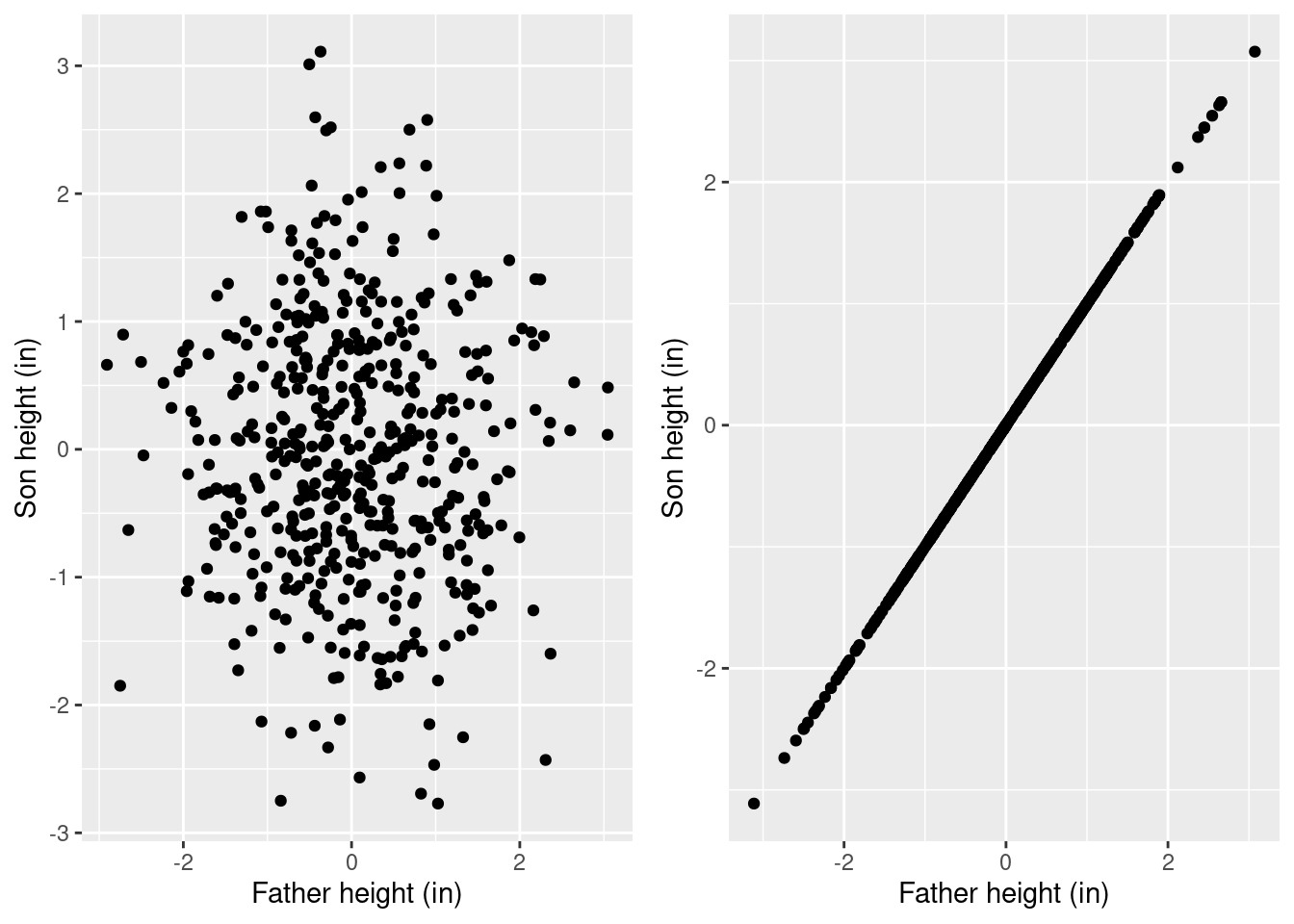
Our real data looks somewhere in between, so we expect a slope of something between \(0\) and \(1\).
However, you can also make the reasoning go the other way!
Although we regressed sons on fathers, we could have equally well regressed fathers on sons, and got exactly the same result. In other words, we have
\[ \expect{h_{n2} \vert h_{n1}} = \beta h_{n1} \quad\textrm{and}\quad \expect{h_{n1} \vert h_{n2}} = \beta h_{n2}, \]
for roughly the same \(\beta < 1\). Note that without the expectations this would be impossible! In fact, by ordinary algebra, if
\[ h_{n2} = \beta h_{n1} \quad\Rightarrow\quad h_{n1} = \beta^{-1} h_{n2}. \]
If \(0 < \beta < 1\), then we must have \(\beta^{-1} > 1\), in contradiction to our regression result. Mixing up the expectation estimated by regression and a deterministic algebraic result is the source of what may seem paradoxical about regression to the mean.
Regression to the mean due to stationarity
Imagine a sequence of generations of fathers and sons numbered \(1,2,3\ldots\). Let the height of the individual in generation \(i\) be \(h_i\). Specifically, \(h_1, h_2\) form a father–son pair of heights.
Suppose that the marginal variance of heights is constant. Without loss of generality, we can take \(\var{h_i} = 1\) for all \(i\). For simplicity, we can also assume that \(\expect{h_i} = 0\), so that heights are measured relative to the overall mean.
What does this mean about the conditional mean \(\expect{h_{i + 1} | h_{i}}\)? Suppose that \(\expect{h_{i + 1} \vert h_{i}} = \beta h_{i}\), meaning that, on average, a son’s height is \(\beta\) times the father’s height.
\[ \begin{aligned} 1 ={}& \var{h_2} \\={}& \expect{h_2^2} \\={}& \expect{\expect{h_2^2 | h_1}} \\={}& \expect{\expect{h_2^2 | h_1} - \expect{h_2 \vert h_1}^2 + \expect{h_2 \vert h_1}^2} \\={}& \expect{\var{h_2 | h_1}} + \expect{(\beta h_1)^2} \\={}& \expect{\var{h_2 | h_1}} + \beta^2 \expect{h_1^2} \\={}& \expect{\var{h_2 | h_1}} + \beta^2 \Rightarrow\\ \beta ={}& \sqrt{1 - \expect{\var{h_2 | h_1}}}. \end{aligned} \]
This means that as long as there is some variability in the son’s height given the father (so \(\expect{\var{h_2 | h_1}} > 0\)), then \(\beta\) must be less than one, otherwise the variance of heights would be growing over time.
Regression to the mean as errors in variables
This motivates a different perspective on the same problem: errors in variables. Rather than modeling \(\expect{h_{i+ 1} | h_i}\) directly, a more reasonable model is that both \(h_i\) and \(h_{i + 1}\) are noisy measurements of the same quantity.
Suppose that fathers and sons come from a “lineage” \(n\), with heights \(h_{n1}\) and \(h_{n2}\) respectively. Let’s say that the father and son share a genetic propensity for tallness, \(\mu_n\), and that
\[ h_{n1} = \mu_n + \res_{n1} \quad\textrm{and}\quad h_{n2} = \mu_n + \res_{n2}, \]
where \(\res_{n1}\) and \(\res_{n2}\) are IID mean zero “errors,” or deviations from the shared “propensity.” If \(\mu_n\) is IID across \(m\) and independent of the errors, then
\[ \var{h_{ni}} = \var{\mu_n} + \var{\res_{n1}} = \sigma_\mu^2 + \sigma_\res^2 = 1 \]
so the “total” marginal variance of heights is decomposed into a component due to the variability in genetics (\(\sigma_\mu^2\))and the ideosyncratic variability of individuals (\(\sigma_\res^2\)). Note that
\[ \expect{h_{n1} | m} = \expect{h_{n2} | \textrm{lineage }n} = \mu_n, \]
so sons and fathers are the same height on average. However, if we regress \(h_{n2} \sim \beta h_{n1}\), we get
\[ \begin{aligned} \betahat ={}& \frac{\meann h_{n2} h_{n1}}{ \meann h_{n1}^2} \\={}& \frac{\meann (\mu_n + \res_{n2}) (\mu_n + \res_{n2}) } { \meann (\mu_n + \res_{n1})^2} \\={}& \frac{\meann \mu_n^2 + \meann \res_{n2} \mu_n + \meann \res_{n1} \mu_n + \meann \res_{n1} \res_{n2} } {\meann \mu_n^2 + \meann \res_{n1} \mu_n + \meann \res_{n1} \mu_n + \meann \res_{n1}^2 } \\\approx{}& \frac{\sigma_\mu^2}{\sigma_\mu^2 + \sigma_\res^2} < 1. \end{aligned} \]
Again, we see that \(\betahat\) must be less than one as long as there is some ideosyncratic variation, \(\sigma_\res^2 > 0\).
Error in variables more generally
In fact, regression to the mean is a special case of a more general phenomenon of “errors in regressors.” In general, the problem looks like this.
Suppose you believe that \(\y_n = \betav^\trans \xv_n + \res_n\), but you don’t observe \(\xv_n\) directly. Instead, you observe
\[ \zv_n = \xv_n + \etav_n, \]
where \(\etav\) is a mean zero random error independent of everything else (in particular, of \(\res_n\)).
What happens if you regress \(\y_n \sim \gammav^\trans \zv_n\) instead of \(\xv_n\)? The answer is you bias the estimate of \(\beta\) by an amount determined by the covariance of \(\etav_n\). Specifically, if \(\etav_n\) has covariance \(\cov(\etav_n) = \V\), then
\[ \begin{aligned} \gammav ={}& \left(\Z^\trans \Z \right)^{-1} \Z^\trans \Y \\={}& \left((\X + \etav)^\trans (\X + \etav) \right)^{-1} (\X + \etav)^\trans (\X \betav + \resv) \\={}& \left(\frac{1}{N}\left(\X^\trans \X + \X^\trans \etav + \etav^\trans \X + \etav^\trans \etav \right) \right)^{-1} \frac{1}{N} \left(\X^\trans \X \betav + \etav^\trans \X \betav + \X^\trans \resv + \etav^\trans \resv \right). \\\approx{}& \left(\frac{1}{N} \X^\trans \X + \V \right)^{-1} \frac{1}{N} \X^\trans \X \betav. \end{aligned} \]