git_repo_dir <- "/home/rgiordan/Documents/git_repos/stat151a"
housing_dir <- file.path(git_repo_dir, "datasets/ames_house/data")
ames_orig <- read.table(file.path(housing_dir, "AmesHousing.txt"), sep="\t", header=T)Multilinear regression with the Ames Housing data
Dataset
We will take a look at the Ames housing data from Veridical Data Science by Yu and Barter. It is also available on the course website in the datasets page. (The original data is on github.)
These are a sample of homes sold in Ames Iowas between 2006 and 2010 as recorded by the city assessor’s office. See the discussion in Chapter 8.4 of VDS..
We will be looking at this data to ask the question: how much might I increase my home’s value by renovating the kitchen?
The dataset lists sale price, as well as different “kitchen quality” measures:
KitchenQual (Ordinal): Kitchen quality
       Ex       Excellent
       Gd       Good
       TA       Typical/Average
       Fa       Fair
Po PoorWe will follow some of the cleaning suggestions in the VDS book.
We’ll also look only at “good” and “excellent” kitchens, on the assumption that we are upgrading our kitchen from its present “good” condtion to “excellent.”
ames <- ames_orig %>%
  filter(Sale.Condition == "Normal",
         # remove agricultural, commercial and industrial
         !(MS.Zoning %in% c("A (agr)", "C (all)", "I (all)"))) %>%
  filter(Kitchen.Qual %in% c("Gd", "Ex")) %>%
mutate(Overall.Qual=factor(Overall.Qual))ggplot(ames) +
geom_histogram(aes(x=SalePrice), bins=50)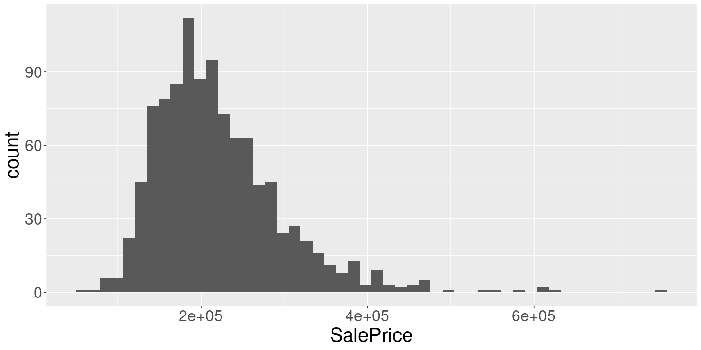
Inference
One way we might ask much we increase the home’s value by upgrading the kitchen is to look at the mean sales price for both good and excellent kitchens.
ames %>%
  ggplot() +
      geom_boxplot(aes(x=Kitchen.Qual, y=SalePrice, fill=Kitchen.Qual))+
      expand_limits(y=0)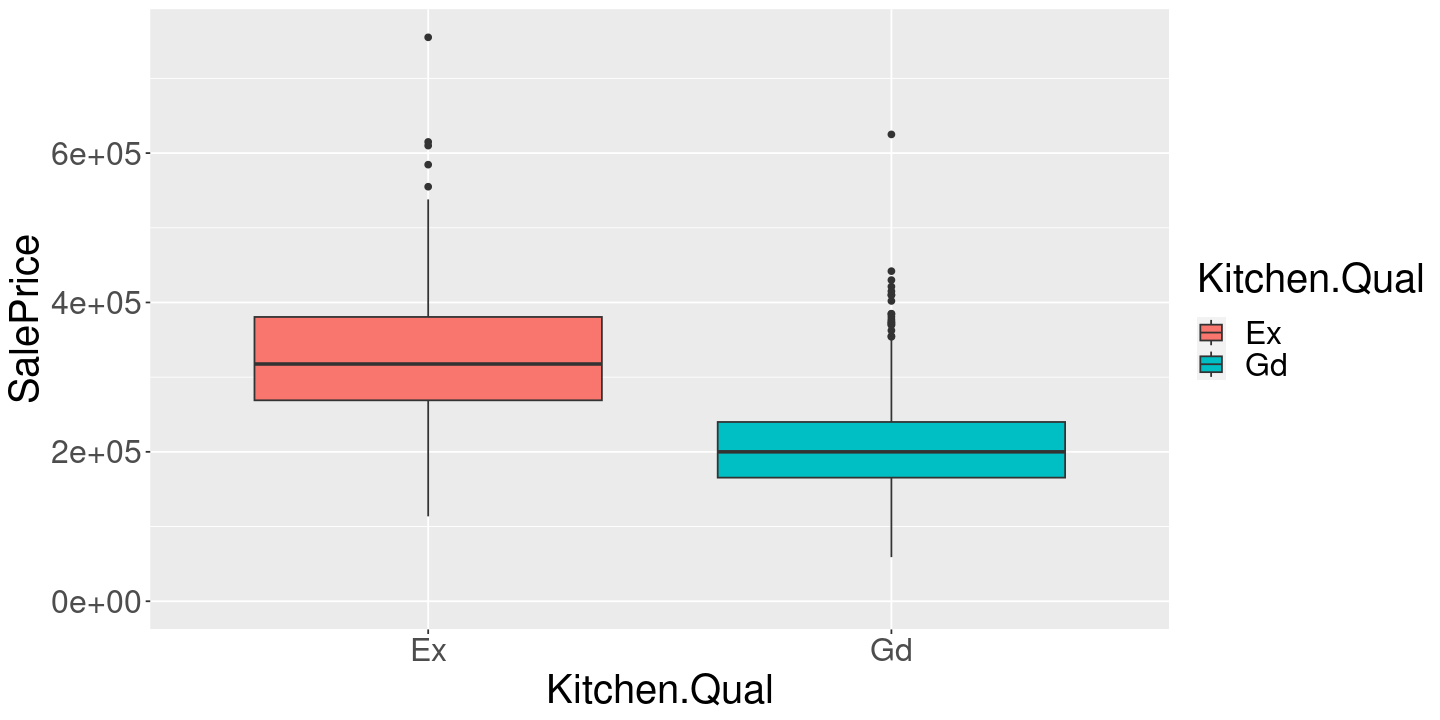
mean_diff <-
    ames %>%
        group_by(Kitchen.Qual) %>%
        summarize(mean_price=mean(SalePrice)) %>%
        pivot_wider(names_from=Kitchen.Qual, values_from=mean_price) %>%
        mutate(difference=Ex - Gd)

print(mean_diff)
# A tibble: 1 × 3
Ex Gd difference
<dbl> <dbl> <dbl>
1 327007. 207828. 119179.The difference is quite large! Maybe upgrading your kitchen is a great investment.
Viewing the difference of means as a regression
Note that we can compute the same thing with a regression.
reg <- lm(SalePrice ~ Kitchen.Qual - 1, ames)
print(summary(reg))
Call:
lm(formula = SalePrice ~ Kitchen.Qual - 1, data = ames)

Residuals:
    Min      1Q  Median      3Q     Max
-213307  -44953   -7878   35297  427993

Coefficients:
               Estimate Std. Error t value Pr(>|t|)
Kitchen.QualEx   327006       6305   51.87   <2e-16 ***
Kitchen.QualGd   207828       2215   93.83   <2e-16 ***
---
Signif. codes:  0 ‘***’ 0.001 ‘**’ 0.01 ‘*’ 0.05 ‘.’ 0.1 ‘ ’ 1

Residual standard error: 67910 on 1054 degrees of freedom
Multiple R-squared:  0.916, Adjusted R-squared:  0.9158
F-statistic:  5747 on 2 and 1054 DF,  p-value: < 2.2e-16
What is going on? When we run the regression, R is converting Kitchen.Qual into a binary matrix.
x <- model.matrix(SalePrice ~ Kitchen.Qual - 1, ames)

bind_cols(
    select(ames, Kitchen.Qual),
    x) %>%
head(, 10)| Kitchen.Qual | Kitchen.QualEx | Kitchen.QualGd | |
|---|---|---|---|
| <chr> | <dbl> | <dbl> | |
| 1 | Gd | 0 | 1 |
| 2 | Ex | 1 | 0 |
| 3 | Gd | 0 | 1 |
| 4 | Gd | 0 | 1 |
| 5 | Gd | 0 | 1 |
| 6 | Gd | 0 | 1 |
We then find the coefficients \(\beta_{ex}\) and \(\beta_{gd}\) that minimizes
\[ \sum_{n=1}^N (y_n - (\beta_{ex} \textrm{Kitchen.QualEx} + \beta_{gd} \textrm{Kitchen.QualGd}))^2 \]
where \(y_n =\)SalePrice.
Exercise: prove that the optimal values, \(\hat\beta_{ex}\) and \(\hat\beta_{gd}\), are just the sample means within their respective categories, e.g.
\[ \hat\beta_{ex} = \frac{1}{N_{ex}} \sum_{n: \textrm{Kitchen.Qual} = \textrm{Ex}} y_n \]
There are a couple ways to get the difference out of R.
predict(reg, data.frame(Kitchen.Qual="Ex")) - predict(reg, data.frame(Kitchen.Qual="Gd"))betahat <- coefficients(reg)
diff <- betahat["Kitchen.QualEx"] - betahat["Kitchen.QualGd"]
names(diff) <- NULL
print(diff)[1] 119178.5Here’s one you might not have thought of:
reg2 <- lm(SalePrice ~ Kitchen.Qual + 1, ames)
print(summary(reg2))
Call:
lm(formula = SalePrice ~ Kitchen.Qual + 1, data = ames)

Residuals:
    Min      1Q  Median      3Q     Max
-213307  -44953   -7878   35297  427993

Coefficients:
               Estimate Std. Error t value Pr(>|t|)
(Intercept)      327006       6305   51.87   <2e-16 ***
Kitchen.QualGd  -119178       6683  -17.83   <2e-16 ***
---
Signif. codes:  0 ‘***’ 0.001 ‘**’ 0.01 ‘*’ 0.05 ‘.’ 0.1 ‘ ’ 1

Residual standard error: 67910 on 1054 degrees of freedom
Multiple R-squared:  0.2318,    Adjusted R-squared:  0.2311
F-statistic:   318 on 1 and 1054 DF,  p-value: < 2.2e-16
Here, the model includes a constant, which is always 1. Then it includes an encoding vector only for Kitchen.QualGd.
Exercise: Why doesn’t it include one for Kitchen.QualEx?
x <- model.matrix(SalePrice ~ Kitchen.Qual + 1, ames)

bind_cols(
    select(ames, Kitchen.Qual),
    x) %>%
head(, 10)| Kitchen.Qual | (Intercept) | Kitchen.QualGd | |
|---|---|---|---|
| <chr> | <dbl> | <dbl> | |
| 1 | Gd | 1 | 1 |
| 2 | Ex | 1 | 0 |
| 3 | Gd | 1 | 1 |
| 4 | Gd | 1 | 1 |
| 5 | Gd | 1 | 1 |
| 6 | Gd | 1 | 1 |
predict(reg2, data.frame(Kitchen.Qual="Ex")) - predict(reg2, data.frame(Kitchen.Qual="Gd"))One way to interpret this is “what is the effect on sale price of having a good kitchen when controlling for the average home price?”
Controlling for house quality
We also have a measure of overall house quality:
Overall Qual (Ordinal): Rates the overall material and finish of the house

       10       Very Excellent
       9        Excellent
       8        Very Good
       7        Good
       6        Above Average
       5        Average
       4        Below Average
       3        Fair
       2        Poor
       1        Very Poor
If we have discovered the “true effect of remodeling your kitchen” then the difference in sales price should not depend on the overall house condition, right? (After all, I haven’t said what my house condition is when I asked the question.) Let’s see.
ames %>%
  ggplot() +
  geom_boxplot(aes(x=Kitchen.Qual, y=SalePrice, fill=Kitchen.Qual)) +
  facet_grid( ~ Overall.Qual)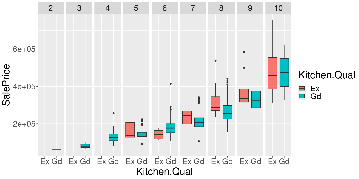
ames %>%
    group_by(Overall.Qual, Kitchen.Qual) %>%
    summarize(mean_price=mean(SalePrice), .groups="drop") %>%
    pivot_wider(id_cols=Overall.Qual, names_from=Kitchen.Qual, values_from=mean_price) %>%
mutate(difference=Ex - Gd)| Overall.Qual | Gd | Ex | difference |
|---|---|---|---|
| <fct> | <dbl> | <dbl> | <dbl> |
| 2 | 59000.0 | NA | NA |
| 3 | 81100.0 | NA | NA |
| 4 | 132468.4 | NA | NA |
| 5 | 146430.7 | 169931.2 | 23500.598 |
| 6 | 180235.6 | 142425.0 | -37810.618 |
| 7 | 209187.3 | 239900.0 | 30712.678 |
| 8 | 263591.5 | 311165.7 | 47574.197 |
| 9 | 328735.8 | 355043.4 | 26307.578 |
| 10 | 475000.0 | 478246.2 | 3246.154 |
This not only gives a very different answer to our original difference in means, but it even gives surprising answers, such as a negative value for a particular value of overall quality.
Exercise: How can you explain the difference in these results?
How can we compute these separate means as regression?
reg_qual <- lm(SalePrice ~ Overall.Qual : Kitchen.Qual - 1, ames)
print(summary(reg_qual))
Call:
lm(formula = SalePrice ~ Overall.Qual:Kitchen.Qual - 1, data = ames)

Residuals:
    Min      1Q  Median      3Q     Max
-168246  -29701   -4211   22776  276754

Coefficients: (3 not defined because of singularities)
                              Estimate Std. Error t value Pr(>|t|)
Overall.Qual2:Kitchen.QualEx        NA         NA      NA       NA
Overall.Qual3:Kitchen.QualEx        NA         NA      NA       NA
Overall.Qual4:Kitchen.QualEx        NA         NA      NA       NA
Overall.Qual5:Kitchen.QualEx    169931      16713  10.168  < 2e-16 ***
Overall.Qual6:Kitchen.QualEx    142425      23636   6.026 2.33e-09 ***
Overall.Qual7:Kitchen.QualEx    239900      13646  17.580  < 2e-16 ***
Overall.Qual8:Kitchen.QualEx    311166       9271  33.565  < 2e-16 ***
Overall.Qual9:Kitchen.QualEx    355043       6493  54.679  < 2e-16 ***
Overall.Qual10:Kitchen.QualEx   478246      13111  36.478  < 2e-16 ***
Overall.Qual2:Kitchen.QualGd     59000      47271   1.248  0.21227
Overall.Qual3:Kitchen.QualGd     81100      27292   2.972  0.00303 **
Overall.Qual4:Kitchen.QualGd    132468      10845  12.215  < 2e-16 ***
Overall.Qual5:Kitchen.QualGd    146431       4408  33.219  < 2e-16 ***
Overall.Qual6:Kitchen.QualGd    180236       3286  54.857  < 2e-16 ***
Overall.Qual7:Kitchen.QualGd    209187       2491  83.964  < 2e-16 ***
Overall.Qual8:Kitchen.QualGd    263592       3173  83.083  < 2e-16 ***
Overall.Qual9:Kitchen.QualGd    328736      14253  23.065  < 2e-16 ***
Overall.Qual10:Kitchen.QualGd   475000      33426  14.211  < 2e-16 ***
---
Signif. codes:  0 ‘***’ 0.001 ‘**’ 0.01 ‘*’ 0.05 ‘.’ 0.1 ‘ ’ 1

Residual standard error: 47270 on 1041 degrees of freedom
Multiple R-squared:  0.9598,    Adjusted R-squared:  0.9592
F-statistic:  1657 on 15 and 1041 DF,  p-value: < 2.2e-16
We can see that the estimates are the same as the means.
Let’s look at the regressor matrix that we’re constructing:
x <- model.matrix(SalePrice ~ Overall.Qual : Kitchen.Qual - 1, ames)

bind_cols(
    select(ames, SalePrice, Overall.Qual, Kitchen.Qual),
    x) %>%
head(15) %>% t()| 1 | 2 | 3 | 4 | 5 | 6 | 7 | 8 | 9 | 10 | 11 | 12 | 13 | 14 | 15 | |
|---|---|---|---|---|---|---|---|---|---|---|---|---|---|---|---|
| SalePrice | 172000 | 244000 | 195500 | 213500 | 191500 | 236500 | 189000 | 171500 | 212000 | 538000 | 216000 | 184000 | 149900 | 306000 | 275000 |
| Overall.Qual | 6 | 7 | 6 | 8 | 8 | 8 | 7 | 7 | 8 | 8 | 7 | 7 | 6 | 8 | 9 |
| Kitchen.Qual | Gd | Ex | Gd | Gd | Gd | Gd | Gd | Gd | Gd | Ex | Gd | Gd | Gd | Gd | Ex |
| Overall.Qual2:Kitchen.QualEx | 0 | 0 | 0 | 0 | 0 | 0 | 0 | 0 | 0 | 0 | 0 | 0 | 0 | 0 | 0 |
| Overall.Qual3:Kitchen.QualEx | 0 | 0 | 0 | 0 | 0 | 0 | 0 | 0 | 0 | 0 | 0 | 0 | 0 | 0 | 0 |
| Overall.Qual4:Kitchen.QualEx | 0 | 0 | 0 | 0 | 0 | 0 | 0 | 0 | 0 | 0 | 0 | 0 | 0 | 0 | 0 |
| Overall.Qual5:Kitchen.QualEx | 0 | 0 | 0 | 0 | 0 | 0 | 0 | 0 | 0 | 0 | 0 | 0 | 0 | 0 | 0 |
| Overall.Qual6:Kitchen.QualEx | 0 | 0 | 0 | 0 | 0 | 0 | 0 | 0 | 0 | 0 | 0 | 0 | 0 | 0 | 0 |
| Overall.Qual7:Kitchen.QualEx | 0 | 1 | 0 | 0 | 0 | 0 | 0 | 0 | 0 | 0 | 0 | 0 | 0 | 0 | 0 |
| Overall.Qual8:Kitchen.QualEx | 0 | 0 | 0 | 0 | 0 | 0 | 0 | 0 | 0 | 1 | 0 | 0 | 0 | 0 | 0 |
| Overall.Qual9:Kitchen.QualEx | 0 | 0 | 0 | 0 | 0 | 0 | 0 | 0 | 0 | 0 | 0 | 0 | 0 | 0 | 1 |
| Overall.Qual10:Kitchen.QualEx | 0 | 0 | 0 | 0 | 0 | 0 | 0 | 0 | 0 | 0 | 0 | 0 | 0 | 0 | 0 |
| Overall.Qual2:Kitchen.QualGd | 0 | 0 | 0 | 0 | 0 | 0 | 0 | 0 | 0 | 0 | 0 | 0 | 0 | 0 | 0 |
| Overall.Qual3:Kitchen.QualGd | 0 | 0 | 0 | 0 | 0 | 0 | 0 | 0 | 0 | 0 | 0 | 0 | 0 | 0 | 0 |
| Overall.Qual4:Kitchen.QualGd | 0 | 0 | 0 | 0 | 0 | 0 | 0 | 0 | 0 | 0 | 0 | 0 | 0 | 0 | 0 |
| Overall.Qual5:Kitchen.QualGd | 0 | 0 | 0 | 0 | 0 | 0 | 0 | 0 | 0 | 0 | 0 | 0 | 0 | 0 | 0 |
| Overall.Qual6:Kitchen.QualGd | 1 | 0 | 1 | 0 | 0 | 0 | 0 | 0 | 0 | 0 | 0 | 0 | 1 | 0 | 0 |
| Overall.Qual7:Kitchen.QualGd | 0 | 0 | 0 | 0 | 0 | 0 | 1 | 1 | 0 | 0 | 1 | 1 | 0 | 0 | 0 |
| Overall.Qual8:Kitchen.QualGd | 0 | 0 | 0 | 1 | 1 | 1 | 0 | 0 | 1 | 0 | 0 | 0 | 0 | 1 | 0 |
| Overall.Qual9:Kitchen.QualGd | 0 | 0 | 0 | 0 | 0 | 0 | 0 | 0 | 0 | 0 | 0 | 0 | 0 | 0 | 0 |
| Overall.Qual10:Kitchen.QualGd | 0 | 0 | 0 | 0 | 0 | 0 | 0 | 0 | 0 | 0 | 0 | 0 | 0 | 0 | 0 |
Controlling for living area
We might ask the same question about living area. Unfortunately this is now a continuous variable.
ames %>%
    ggplot() +
      geom_histogram(aes(x=Gr.Liv.Area), bins=40)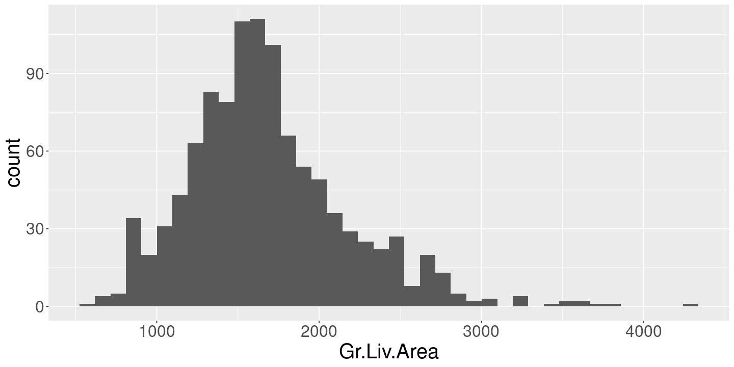
It no longer makes sense to look at the difference in means “for a fixed living area,” as you can see by the scatter plot.
ames %>%
  ggplot() +
  geom_point(aes(x=Gr.Liv.Area, y=SalePrice, color=Kitchen.Qual)) +
  expand_limits(y=0)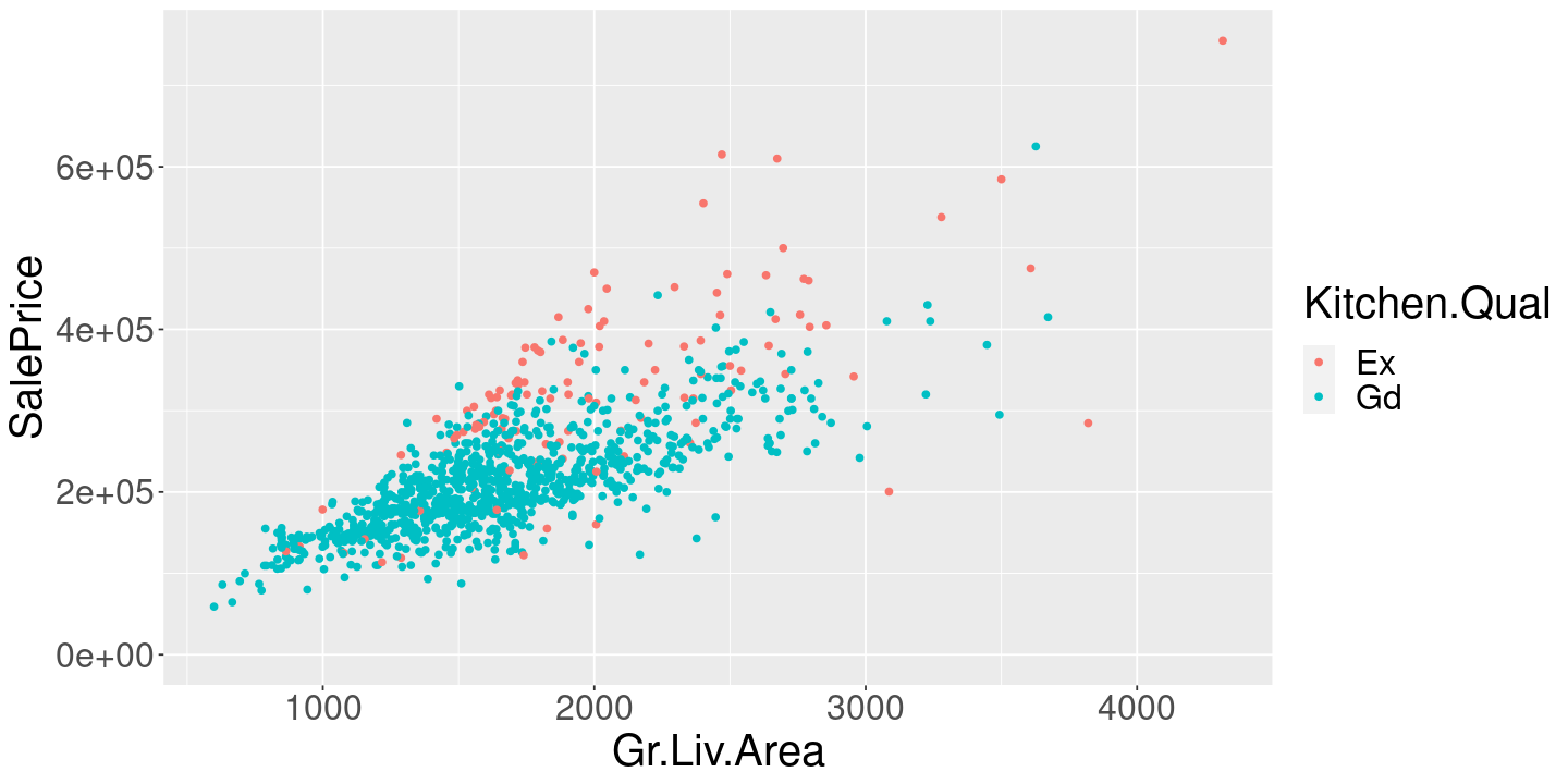
ames %>%
    mutate(LivingAreaBin=cut(Gr.Liv.Area, 10)) %>%
    ggplot() +
        geom_boxplot(aes(x=Kitchen.Qual, y=SalePrice, fill=Kitchen.Qual)) +
        facet_grid( ~ LivingAreaBin)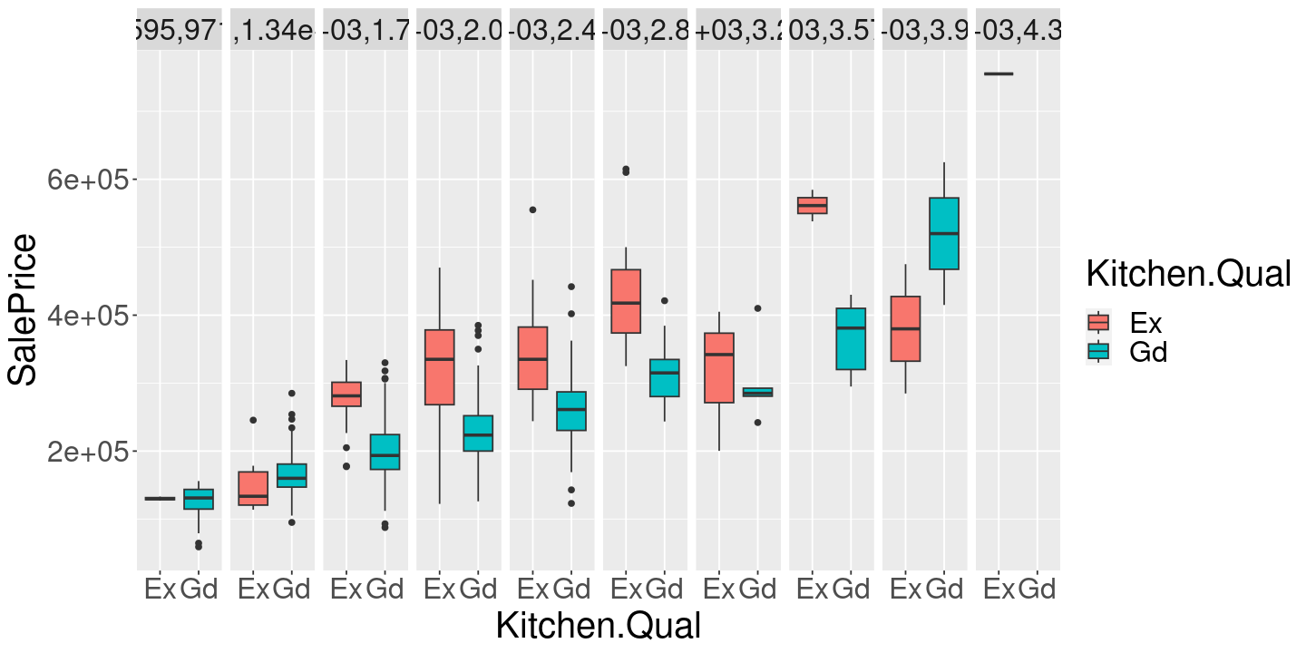
reg_la <- lm(SalePrice ~ Gr.Liv.Area + Kitchen.Qual, ames)
print(summary(reg_la))

ames %>%
    mutate(PredPrice=predict(reg_la, ames)) %>%
  ggplot() +
      geom_point(aes(x=Gr.Liv.Area, y=SalePrice, color=Kitchen.Qual)) +
      geom_line(aes(x=Gr.Liv.Area, y=PredPrice, color=Kitchen.Qual, group=Kitchen.Qual), lwd=2) +
      expand_limits(y=0)
Call:
lm(formula = SalePrice ~ Gr.Liv.Area + Kitchen.Qual, data = ames)

Residuals:
    Min      1Q  Median      3Q     Max
-238658  -24841   -2552   23240  240508

Coefficients:
                 Estimate Std. Error t value Pr(>|t|)
(Intercept)    115200.021   7234.776   15.92   <2e-16 ***
Gr.Liv.Area       104.977      2.912   36.05   <2e-16 ***
Kitchen.QualGd -79532.676   4606.565  -17.27   <2e-16 ***
---
Signif. codes:  0 ‘***’ 0.001 ‘**’ 0.01 ‘*’ 0.05 ‘.’ 0.1 ‘ ’ 1

Residual standard error: 45460 on 1053 degrees of freedom
Multiple R-squared:  0.6561,    Adjusted R-squared:  0.6555
F-statistic:  1005 on 2 and 1053 DF,  p-value: < 2.2e-16

Taking this seriously, we might estimate that the coefficient on Kitchen.QualGd tells us the answer to our question. But the modeling assumptions to not look reasonable. Note, for example, the particularly bad fit of the Ex line for low living area houses.
Controlling for too much
Furthermore, we can even further subdivide and try to “control” for overall quality and living area simultaneously. This is probably closer to what we actually want, but we have real problems with data sparsity now.
options(repr.plot.width=20, repr.plot.height=6)
ames %>%
  ggplot() +
  geom_point(aes(x=Gr.Liv.Area, y=SalePrice, color=Kitchen.Qual)) +
  facet_grid( ~ Overall.Qual) +
  expand_limits(y=0) +
  theme(axis.text.x = element_text(angle = 90, vjust = 0.5, hjust=1))
options(repr.plot.width=12, repr.plot.height=6)
This is getting difficult. What about a linear model?
big_reg <-
    lm(SalePrice ~ Gr.Liv.Area + Kitchen.Qual + Overall.Qual, ames)

print(summary(big_reg))
Call:
lm(formula = SalePrice ~ Gr.Liv.Area + Kitchen.Qual + Overall.Qual,
    data = ames)

Residuals:
    Min      1Q  Median      3Q     Max
-143175  -19875   -1192   18301  150483

Coefficients:
                 Estimate Std. Error t value Pr(>|t|)
(Intercept)     32630.906  34316.248   0.951  0.34188
Gr.Liv.Area        77.251      2.451  31.524  < 2e-16 ***
Kitchen.QualGd -19904.252   4506.865  -4.416 1.11e-05 ***
Overall.Qual3   12932.882  39229.663   0.330  0.74171
Overall.Qual4   17359.803  34900.926   0.497  0.61901
Overall.Qual5   35439.120  34151.188   1.038  0.29964
Overall.Qual6   49218.494  34127.289   1.442  0.14954
Overall.Qual7   65443.802  34124.965   1.918  0.05541 .
Overall.Qual8  107153.925  34189.871   3.134  0.00177 **
Overall.Qual9  167573.989  34581.308   4.846 1.45e-06 ***
Overall.Qual10 241076.614  35627.832   6.767 2.19e-11 ***
---
Signif. codes:  0 ‘***’ 0.001 ‘**’ 0.01 ‘*’ 0.05 ‘.’ 0.1 ‘ ’ 1

Residual standard error: 33970 on 1045 degrees of freedom
Multiple R-squared:  0.8094,    Adjusted R-squared:  0.8075
F-statistic: 443.7 on 10 and 1045 DF,  p-value: < 2.2e-16
One way to interpret this is via making predictions for a given house, one with a renovated kitchen and one without.
sample_house <-
    filter(ames, Kitchen.Qual == "Gd") %>%
    sample_n(1)

sample_house_reno <- sample_house %>% mutate(Kitchen.Qual="Ex")

predict(big_reg, sample_house_reno) - predict(big_reg, sample_house) Of course, the problem is that we may get different answers depending on what regression we run:
lm(SalePrice ~ Gr.Liv.Area + Kitchen.Qual, ames) %>%
    summary()
Call:
lm(formula = SalePrice ~ Gr.Liv.Area + Kitchen.Qual, data = ames)

Residuals:
    Min      1Q  Median      3Q     Max
-238658  -24841   -2552   23240  240508

Coefficients:
                 Estimate Std. Error t value Pr(>|t|)
(Intercept)    115200.021   7234.776   15.92   <2e-16 ***
Gr.Liv.Area       104.977      2.912   36.05   <2e-16 ***
Kitchen.QualGd -79532.676   4606.565  -17.27   <2e-16 ***
---
Signif. codes:  0 ‘***’ 0.001 ‘**’ 0.01 ‘*’ 0.05 ‘.’ 0.1 ‘ ’ 1

Residual standard error: 45460 on 1053 degrees of freedom
Multiple R-squared:  0.6561,    Adjusted R-squared:  0.6555
F-statistic:  1005 on 2 and 1053 DF,  p-value: < 2.2e-16
Prediction
What if we just asked a different question: can we predict the cost of a house using kitchen quality?
ames %>%
  ggplot() +
      geom_boxplot(aes(x=Kitchen.Qual, y=SalePrice, fill=Kitchen.Qual))+
      expand_limits(y=0)
all_rows <- 1:nrow(ames)
train_rows <- sample(all_rows, floor(nrow(ames) / 2), replace=FALSE)
test_rows <- setdiff(all_rows, train_rows)
print(length(train_rows) / nrow(ames)) # Sanity check

ames_train <- ames[train_rows, ]
[1] 0.5means_df <-
ames_train %>%
group_by(Overall.Qual, Kitchen.Qual) %>%
summarize(mean_price=mean(SalePrice), .groups="drop")
overall_mean <- mean(ames_train$SalePrice)
print(means_df)
print(overall_mean)# A tibble: 15 × 3
Overall.Qual Kitchen.Qual mean_price
<fct> <chr> <dbl>
1 2 Gd 59000
2 3 Gd 79000
3 4 Gd 119375
4 5 Ex 186567.
5 5 Gd 145680.
6 6 Ex 152000
7 6 Gd 180786.
8 7 Ex 237000
9 7 Gd 207547.
10 8 Ex 340378.
11 8 Gd 263649.
12 9 Ex 355400
13 9 Gd 280667.
14 10 Ex 427958.
15 10 Gd 475000
[1] 219703.6ames_test <-
ames[test_rows, ] %>%
select(SalePrice, Overall.Qual, Kitchen.Qual) %>%
inner_join(means_df, by=c("Overall.Qual", "Kitchen.Qual")) %>% # Note: drops missing values!
mutate(err_pred=SalePrice - mean_price, err_base=SalePrice - overall_mean) %>%
summarize(rmse_pred=sqrt(mean(err_pred^2)), rmse_base=sqrt(mean(err_base^2)))
print(ames_test) rmse_pred rmse_base
1 49917.46 79545.31Exercise: When we’re doing prediction, do we care whether or not we have found the “true” cost effect of renovating your kitchen?
